October 26, 2018October 26, 2018 by mikechristenson

Elk

Elk is a plugin for Grasshopper running in Rhino. Elk works with .osm files exported from openstreetmap.org to extract 3D modeling data from public map data.

To begin using Elk:

1. Download Elk from food4rhino (you will need an account).

2. Follow Elk’s installation instructions.

3. Restart Rhino and Grasshopper. Verify that Elk has installed properly.

4. Use openstreetmap.org to identify and Export your site as an .osm file. Save the .osm file in a known location.

5. In Grasshopper, from the Params > Primitive panel, insert the File Path component, and from the Extra > Elk2 panel, insert the Location and OSM Data components. Right-click on the OSM Data component to select the Create 3D Buildings option. Connect the components as shown below:

elk-1

6. In Rhino, zoom extents to see the results:

elk-2

October 31, 2016 by mikechristenson

Rhino to AutoCAD Workflow: Cutting a Section

This workflow is designed to generate a line-drawn building section from a Rhino model for use in AutoCAD. It begins with a complete Rhino model and concludes with the AutoCAD drawing.

Step 1. Open the Rhino model:

Step 2: Create a new layer. Give the layer a name like SECTION and a distinctive color. Make this new layer current.

Step 3: In the SECTION layer, draw a line as a guide for the section cut. This line represents the line along which the section will be cut:

Step 4: Type SECTION [enter]. When prompted to Select objects for sections, type ALL [enter]:

Step 5. When prompted to designate the Start of section, click on one endpoint of the guideline. When prompted to designate the End of section, move the mouse to the far side of the objects being cut. (Make sure ORTHO, F8, is turned on if you want to cut the section parallel with the relevant major axis.)

Step 6. Because SECTION is a drawing command, it generates new geometry. As soon as the SECTION command is complete, the newly drawn geometry is automatically highlighted:

Step 7. With the new geometry highlighted, choose File > Export Selected:

Step 8. Save the exported geometry in the AutoCAD (.dwg) format:

Step 9. Choose the 2004 Polylines option:

Step 10. Start AutoCAD and open the drawing exported from Rhino:

Step 11. If prompted with a warning dialog, choose Continue opening DWG file:

Step 12. When the file is opened, it will appear in a “top down” view, so the section will appear like a single line:

Step 13. Type 3DORBIT [enter] to orbit the model into a 3D view:

Step 14. The geometry needs to be rotated to sit “flat” on the x-y plane. Type ROTATE3D:

Step 15. When prompted to Select objects, type ALL [enter] to select all of the objects in the drawing:

Step 16. In order to rotate the geometry in three-dimensional space, a rotational axis with two endpoints must be defined. Click on a point within the drawing to define the first endpoint of this axis:

Step 17. With Ortho (F8) turned on, click on another point within the drawing to indicate the other endpoint of the rotational axis:

Step 18. When prompted to Specify rotation angle, type either 90 [enter] or -90 [enter] depending on whether the geometry needs to rotate clockwise or counterclockwise around the axis. (To correct a mistaken rotation, the command can be undone or repeated with a rotation angle of 180.)

Step 19. Type PLAN [enter]:

Step 20. When prompted, click [enter] to accept the Current coordinate system (i. e., the World coordinate system):

Step 21. It may be necessary to rotate the geometry again, but only in two-dimensional space. In the case shown here, the geometry needs to be rotated by 90 degrees. Type ROTATE [enter] and indicate the rotation angle:

Step 22. The section drawing is ready. It may also be necessary to use the FLATTEN command to project all geometry to the x-y plane:

October 7, 2016 by mikechristenson

Rhino to Revit Workflow: Twisted Tower

This workflow demonstrates the possibility of importing mass models from Rhino into Revit for use as Mass Elements. In turn, Revit Masses can be used as the basis for constructing building elements such as floors and walls.

1. In Rhino, create a simple box with plan dimensions 30’ x 30’ and height 100’.

tower_01

2. Type TWIST [enter]. Follow the prompts to twist the tower.

3. Select the twisted tower by clicking on it. Choose File > Export Selected and export the tower as an ACIS SAT file (.sat extension).

4. In Revit, start a new Project based on the Architectural template, or open an existing Project.

5. Start a new Family based on the Conceptual Mass template.

6. On the Insert tab, Import panel, choose Import CAD and navigate to your .sat file. (Make sure that Files of type is set to show .sat files.) Click Open.

7. On the Insert tab, Family Editor panel, choose Load into Project.

8. Click to place the mass.

9. View the mass in the default 3D view to verify its configuration and size.

10. Switch to an Elevation view. Add Levels corresponding to building floors.

11. Click the mass to select it. On the Modify|Mass tab, Model panel, click Mass Floors.

12. Select the Levels for which you wish to create Mass Floors. (Note: depending on the geometry of your tower, the upper and lower Levels may not reliably create Mass Floors.)

tower_09

13. Proceed to use the tools under Massing & Site > Model by Face to create walls and floors.

September 14, 2016 by mikechristenson

Rhino: Learning Resources

This page includes links to recommended resources for learning Rhino.

BOOKS:

Inside Rhinoceros 5, by Ron K.C. Cheng. This book is general in scope, not specifically focused on architectural modelmaking. It provides clear and detailed step-by-step tutorials. However, on the whole, it is probably better-suited to product designers than architects.

VIDEO TUTORIALS:

Although a few of the tutorials are a couple of years old, Nick Senske’s tutorials on Rhino are some of the best available for architecture students. Find a selection here: http://tinyurl.com/j8bfb29 (full link: https://www.youtube.com/watch?v=yPgMccdh8QU&list=PL4GL4fFi1e9fVRVZlB1CJB5VKwmS5e-V6)

Take a look at Nick’s tutorial on modeling in Rhino based on previously-drawn elevations and floor plans: https://www.youtube.com/watch?v=-eP39RbPYrI

The online tutorials provided by McNeel (the company that makes Rhino) are generally good, although they are not specific to architectural modeling.

https://www.rhino3d.com/tutorials

Kyle Houchens has provided an hour-long tutorial focused on architectural modeling, specifically intended for students already familiar with SketchUp. An hour is a long time, but this tutorial is useful if you want to understand Rhino from this basis. The tutorial is from 2014 but the version of Rhino (v5) is still current as of late 2016.

https://vimeo.com/82431575?simple_building

Digital Toolbox has some very good tutorials on Rhino and Grasshopper, including one tutorial specifically focused on architectural modelmaking. Here are the Rhino links:

http://digitaltoolbox.info/rhinoceros-basic/

http://digitaltoolbox.info/rhinoceros-intermediate/

http://digitaltoolbox.info/rhinoceros-advanced/

http://digitaltoolbox.info/farnsworth-house/

March 3, 2015 by mikechristenson

Step-by-Step: Brick Wall on Curved Path

1. In Rhino: Use the BOX command to construct a “brick” with one corner at 0,0,0. Use the CURVE command to construct an arbitrary curved path. [The Grasshopper definition will stack the “brick” along the curved path.]
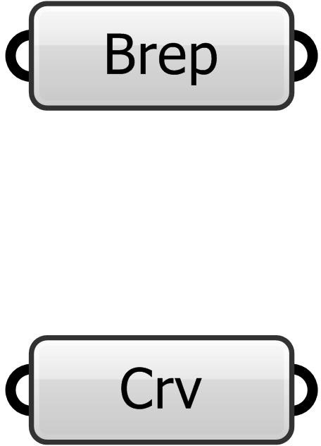
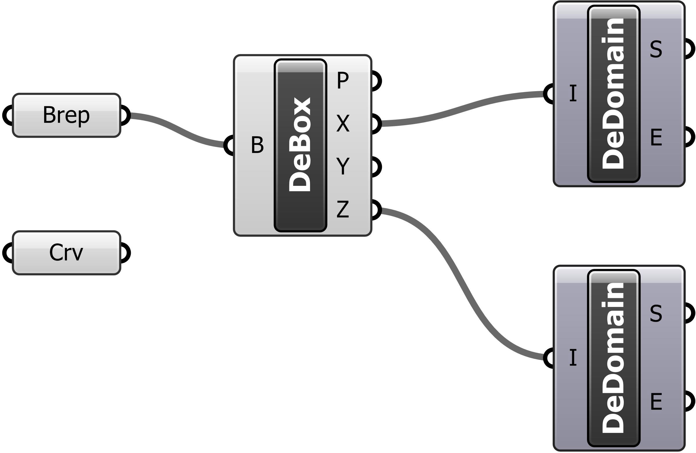
2. Insert the Brep and Crv parameters. Right-click on each in turn to “Set one Brep” and “Set one Curve.”

3. Insert the Deconstruct Box component. Connect the Brep output to the Deconstruct Box input. [Deconstruct Box allows you to measure the X, Y, and Z dimensions of a Box.]

4. Insert two instances of the Deconstruct Domain component. Connect the X output of Deconstruct Box to the input on the first Deconstruct Domain component; connect the Z output of Deconstruct Box to the input on the second Deconstruct Domain component. [Deconstruct Domain extracts the beginning and end points of a domain, in this case the beginning and end points of the X and Z dimensions of the “brick”.]

5. Insert two instances of the Subtraction component. Connect the S output of the first Deconstruct Domain component to the B input of the first Subtraction component; connect the E output of the first Deconstruct Domain component to the A input of the first Subtraction component. Repeat this process with the second Deconstruct Domain and Subtraction components. [The results of the two Subtraction components represent the length and height of the “brick,” respectively.]

6. Insert the Length component and connect it to the Curve component. [This simply measures the length of the Rhino curved path. We will reference it later.]

brick_04
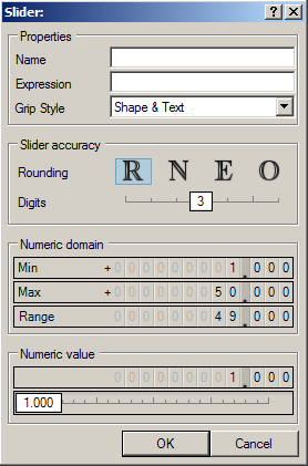
7. Insert a Number Slider. Edit its values as follows: Name: Height. Rounding: Integer Numbers. Numeric domain: Minimum: 1. Maximum: 10.

brick_05
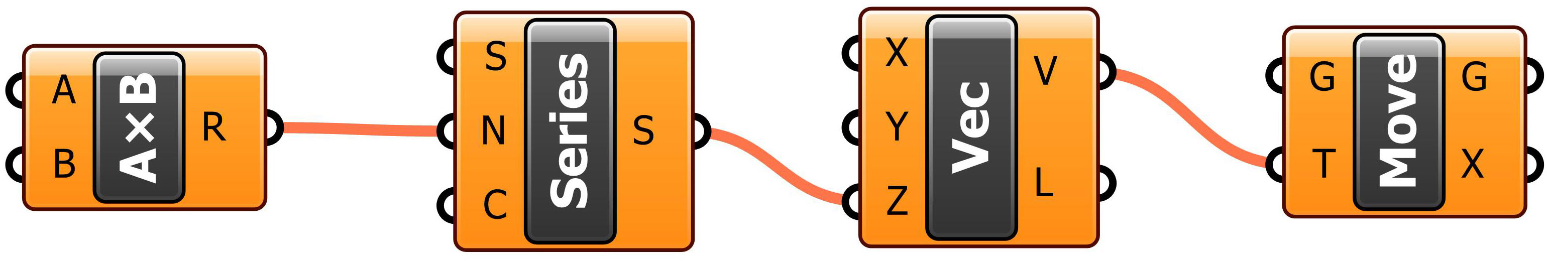
8. On another area on the Canvas, insert the following components: Multiplication, Series, Vector XYZ, and Move. [We will use these components as part of a process to copy the curved path in the vertical direction.]

9. Connect the components: Connect the R output of Multiplication to the N input of Series; connect the S output of Series to the Z input of Vector XYZ; connect the V output of Vector XYZ to the T input of Move.

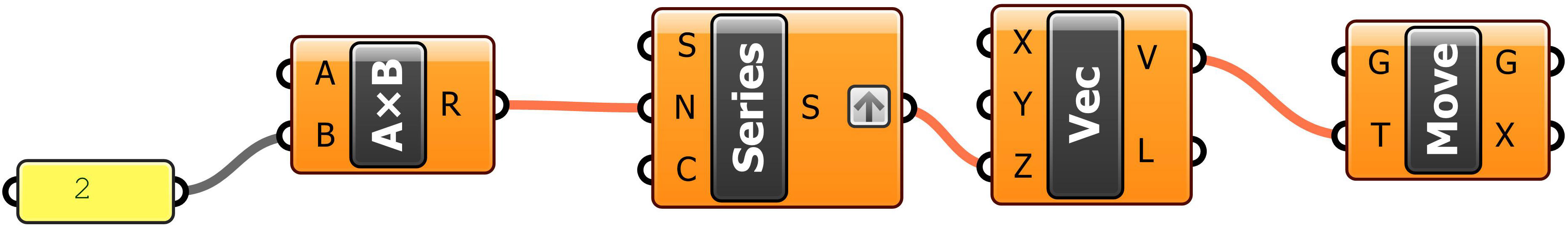
10. Right-click on the S output label of Series and select Graft. [The Graft option changes the data structure of the parameter. Instead of creating a single list of items, it effectively associates each item in a list with a unique source. In our definition, choosing the Graft option will cause Grasshopper to “remember” that the instructions apply to individual bricks.]

11. Insert a Panel component. Edit its value to equal 2, and connect it to the B input of Multiplication.

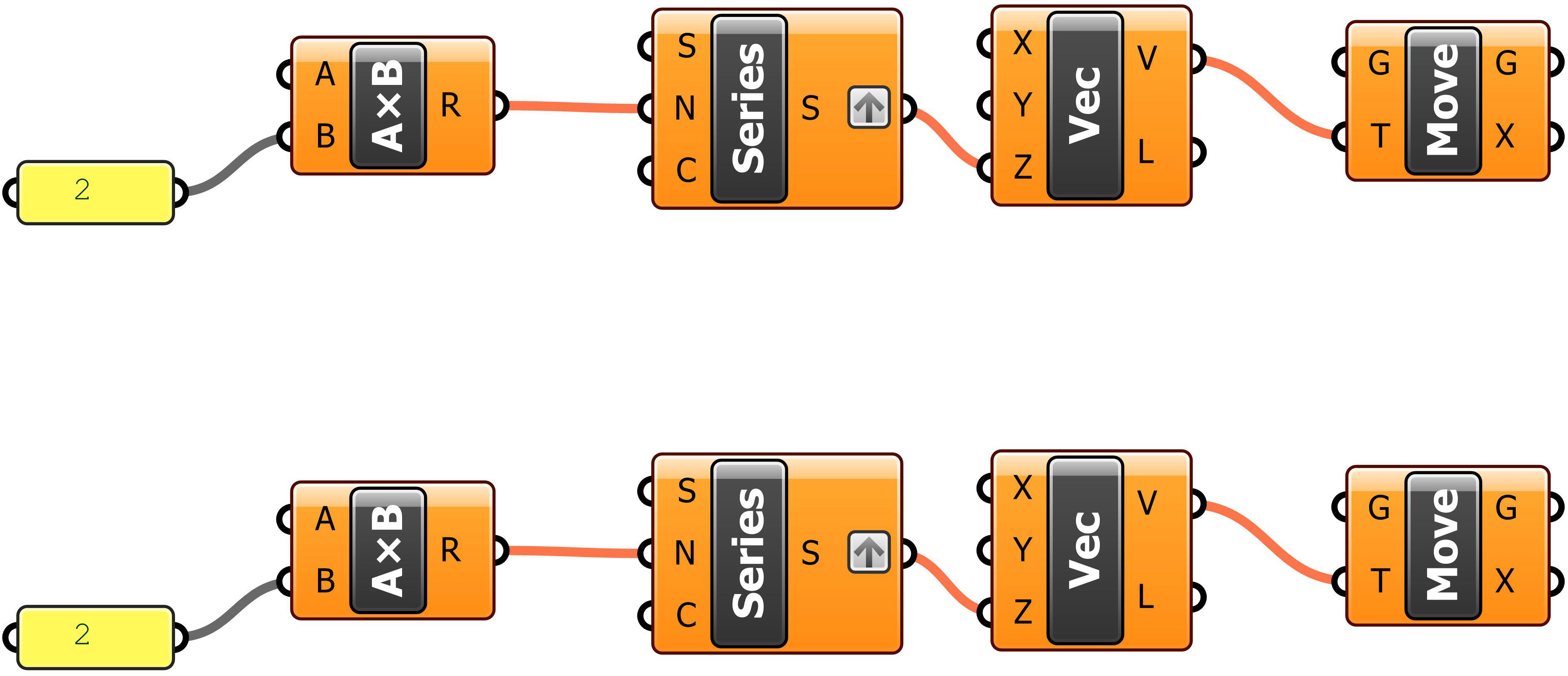
12. Copy-paste this entire group of components (i. e., Panel, Multiplication, Series, Vector XYZ, and Move) and set the new components below the original ones.

13. Connect the components: Refer back to the earlier components we placed. Connect the R output of the second Subtraction component to the A input of each of the Multiplication components (two connections).

14. Connect the components: Again referring back to the earlier components we placed, connect the output of the Number Slider to the C input of each of the Series components (two connections).

15. Insert a Division component. Connect the L output of the Length component (i. e., the Length component which measures the length of the Rhino curve) to the A input of Division. Connect the R output of the first Subtraction component to the B input of Division.

16. On another area on the Canvas, insert the following components: Panel (with a value of 2); Division; Multiplication; Series; Shift List; and Cull Nth. [We will use these components as part of a process to copy the “brick” along the curved path. The Shift List and Cull Nth components are critical to shifting the bricks by half their length on every alternating copy of the curved path.]

17. Connect the components: Panel output to the B input on the Division and Multiplication components; R output of Division to N input on Series; R output of Multiplication to C input of Series; S output of Series to L input of Shift List; L output of Shift List to L input of Cull Nth.

18. Refer back to components placed earlier. Connect the R output of Division (i. e., the Division component connected to the Length component) to the A input of the Multiplication component. Connect the R output of Subtraction (i. e., the first Subtraction component, connected to the Deconstruct Domain component) to the A input of the Division component.

19. Insert a Series component. Connect the R output of Subtraction (i. e., the Subtraction component referred to in the preceding step) to the N input of Series. Connect the R output of Division (i. e., the same Division component referred to in the preceding step) to the C input of Series.

20. On another area of the Canvas, insert the following components: Boolean Toggle, Evaluate Length, and Orient Direction. [The Orient Direction component is responsible for making multiple copies of the original “brick” at the correctly placed and oriented locations along the curved paths.]

21. Connect the components: Output of Boolean Toggle to the N input of Evaluate Length; P output of Evaluate Length to the pB input of Orient Direction; T output of Evaluate Length to the dB input of Orient Direction.

22. Copy-paste this entire group of components (i. e., Boolean Toggle, Evaluate Length, and Orient Direction) and set the new components below the original ones.

23. Insert the following components: Panel (value of 1) and Vector XYZ. Connect the output of Panel to the X input of Vector XYZ, and connect the V output of Vector XYZ to the dA input on each of the Orient Direction components.

24. Refer back to components placed earlier. Connect the Brep (Rhino “brick”) output to the G input on each of the Orient Direction components.

25. Connect the S output of Series (i. e., the Series component placed in step 19) to the L input of the first Evaluate Length component).

26. Connect the G output of Move (i. e., the Move component placed in step 8) to the C input of the first Evaluate Length component).

27. Connect the L output of Cull Nth (i. e., the Cull Nth component placed in step 16) to the L input of the second Evaluate Length component).

28. Connect the G output of Move (i. e., the Move component placed in step 12) to the C input of the second Evaluate Length component).

29. Connect the R output of Subtraction (i. e., the Subtraction component placed in step 5) to the S input of Series (i. e., the Series component placed in step 12).

brick_25a
30. Finally, connect the output on the Crv parameter (i. e., the Rhino “path”) to the G input of each of the Move parameters (i. e., the Move parameters from steps 8 and 12).

31. The definition is complete.

March 1, 2015March 1, 2015 by mikechristenson

Step-by-Step: Lofted Surface Along Curve in Grasshopper

1. In Rhino, use the Curve command to draw an arbitrary curve in 3D space.
2. Start Grasshopper.
3. Insert the Curve parameter.

4. Right-click on the Curve parameter and choose Set one curve. Click on the curve you drew in Rhino.
5. Right-click on the Curve parameter and choose Reparameterize. This forces Grasshopper to measure values along the curve starting with 0 and ending with 1.

6. Insert the Divide Curve component.

7. Insert a Number Slider.

8. Edit the Slider values: Under Slider accuracy, set Integer Numbers. Under Numeric domain, set 1 as the Min and 20 as the Max.

9. Connect the components: Crv output connects to the C input on the Divide Curve component; Slider output connects to the N input on the Divide Curve component. [The first connection tells the Divide Curve component what curve to divide; the second connection tells the Divide Curve component how many divisions to make.]

10. Insert the Circle CNR (Center-Normal-Radius) component.

11. Connect the components: P output on the Divide Curve component connects to the C input on the Circle CNR component; T output on the Divide Curve component connects to the N input on the Circle CNR component. [The first connection tells the Circle CNR component to draw circles centered at each of the division points; the second connection tells the Circle CNR component to “tilt” the planes on which circles are drawn to align with the Rhino curve.]

12. Insert a Loft component.

13. Connect the components: C output on the Circle CNR component connects to the C input on the Loft component. [This connection tells the Loft component to create a surface using the circles as “ribs.”]

14. Insert the Graph Mapper component and another Number Slider.

15. Right-click on the Graph Mapper component. From Graph types, choose SinC.

16. Edit the Slider values: Under Numeric domain, set 1 as the Min and 50 as the Max.

17. Insert the Multiplication component.

18. Connect the components: t output on the Divide Curve component to the input on the Graph Mapper component; output on the Graph Mapper component to the A input on the Multiplication component; output on the Slider to the B input on the Multiplication component. [These connections produce a list of numbers which is then multiplied by the output of the Number Slider. The list of numbers is determined by the y-coordinates of the graph in the Graph Mapper corresponding to the given x-coordinates (i. e., the inputs to the Graph Mapper).]

19. Connect the components: R output on the Multiplication component to the R input on the Circle CNR component. [This connection tells the Circle CNR component to draw circles at radii corresponding to the output of the Multiplication component.]

20. The Grasshopper definition is complete. Experiment by (1) selecting different curves from Rhino; (2) changing the number of divisions (first Number Slider); (3) changing the shape of the graph in the Graph Mapper component (move the grips); (4) changing the graph type in the Graph Mapper component; (5) changing the multiplication value (second Number Slider).

Acknowledgements: This tutorial was inspired by a definition illustrated in the Mode Lab Grasshopper Primer (http://modelab.is/grasshopper-primer/). — Mike Christenson

February 12, 2015February 12, 2015 by mikechristenson

Creating an Emitter Material in Maxwell

Note: Enable Maxwell Fire to see a preview of your render.

If modeling in Rhino:
1. Type LAYER to bring up the Layers palette.
2. In the Layers palette, create a new layer for your emitter material.
3. Click on the Material button next to the layer name.
4. In the Layer Material dialog box, click on the check box next to “Assign material by plug-in: Maxwell for Rhino.”
5. Click Create.
6. Click Edit.
7. In the Material Editor:
a. Give your material a name (e. g., “EMITTER 1”).
b. In the lower left-hand corner of the Material Editor, right-click on BDSF; choose Remove BDSF.
c. In the lower left-hand corner of the Material Editor, right-click on Layer; choose Add Emitter.
d. Under Luminance, you can choose one of several methods for illuminating your Emitter. Depending on the size of the object you are applying the material to, you may need to increase the Watts (or Power). From Maxwell: “It is important to remember that the amount of light emitted from an emitter is spread out across its surface. This means that the same emitter material will look dimmer on a large emitting surface and brighter on a smaller emitting surface.”

Architectural Software

Tag / Rhino

Elk